Building a PyTorch RNN-Based Question Answering System

Overview

• Data Preprocessing and Tokenization
• Architecture Design
• Training Process and Optimization
• Inference and Prediction
• Performance Evaluation and Analysis
• Limitations and Modern Alternatives

Try it out: Below is a live demo of the RNN-based question answering system we'll build in this post. The model is trained on 100 questions and can handle slight variations, but will respond with "I don't know" for questions outside its training data.

Despite the transformer era, understanding Recurrent Neural Networks (RNNs) remains incredibly valuable. RNNs teach the core ideas of sequence modeling—how information flows through time, how representations are built step by step, and how a model can compress a sentence into a compact state that's useful for prediction. Mastering these fundamentals makes modern architectures like LSTMs, GRUs, and transformers far easier to reason about.

In this post, we'll build a minimal but complete RNN-based question answering system in PyTorch—end to end. You'll see how raw text becomes model-ready data, how a small encoder-only RNN turns a question into a fixed-size representation, and how a simple linear layer converts that representation into a single-token answer.

By the end, you’ll understand:

• How to tokenize text and construct a compact vocabulary with <UNK> handling
• How embeddings map token IDs to dense vectors the model can learn from
• How an RNN processes a question over timesteps to accumulate context
• Why we frame answer prediction as classification (not generation) for single-token outputs
• How to train, evaluate, and make predictions with confidence thresholds

This is a hands-on, practical walkthrough. We’ll keep the model intentionally simple so the mechanics are crystal clear, favoring clarity over complexity. Once you grasp these building blocks, you’ll be able to extend the system with LSTM/GRU variants, multi-token generation, or even jump to transformer-based approaches with confidence.

Data Preprocessing and Tokenization

For this RNN based QA system, we will use a dataset of 100 questions and answers 100_Unique_QA_Dataset.csv. You can access the complete implementation and run the code yourself in this Google Colab notebook. To get started, you can follow the steps in Google Colaboratory, first we need to load the dataset in pandas dataframe

import pandas as pd
df = pd.read_csv('/content/100_Unique_QA_Dataset.csv')
df.head()

Expected Output:

Tokenization: Turning Text into Model-Ready Data

Next we have to tokenize the text so that it can be used by the model. To understand the tokenization process, you can refer to one of my previous posts on What is tokenization beyond splitting text? . Tokenziation funciton here is very simple which removes the punctuation and converts the text to lowercase and here is the code for the same.

def tokenize(text):
    text = text.lower()# Convert all characters in the text to lowercase
    text = text.replace('?', '')# Remove question marks from the text
    text = text.replace("'", "")# Remove apostrophes from the text
    text = text.replace("'", "")# Remove apostrophes from the  text
    return text.split()# Split the text into a list of words (tokens) based on whitespace

Building the Vocabulary: Mapping Words to Indices

The vocabulary is the bridge between raw text and the numeric world our model understands. We’ll build a single, unified vocabulary over both questions and answers so the model learns one coherent space of tokens. We’ll also reserve a special <UNK> token for anything unseen at train time, and we’ll keep the mapping bidirectional so we can move from text → indices and back.

# seed the vocabulary with a special token for unknowns
vocab = {"<UNK>": 0}  # ensures unseen tokens map to a safe index

def build_vocab(row):
    tokenized_question = tokenize(row['question'])  # tokenize the question text
    tokenized_answer = tokenize(row['answer'])      # tokenize the answer text
    merged_tokens = tokenized_question + tokenized_answer  # combine both sides to share one vocab

    for token in merged_tokens:                     # iterate over every token in the row
        if token not in vocab:                      # add only if the token is new
            vocab[token] = len(vocab)               # assign the next available integer id

# scan all rows to grow the vocabulary dynamically
df.apply(build_vocab, axis=1)  # applies build_vocab to each row (question, answer)

# create the reverse mapping for decoding indices back to tokens
idx_to_token = {idx: tok for tok, idx in vocab.items()}  # enables numbers → text

These vocabulary design choices work together to create a robust and efficient system. The unified vocabulary approach means the model sees the same token ID regardless of whether it appears in a question or an answer, which simplifies the learning process since the model doesn't need to learn separate representations for the same word in different contexts. The <UNK> token acts as a safety net, ensuring that anything not seen during training still maps to a valid ID instead of crashing the pipeline when we encounter new words. Our dynamic growth strategy keeps the vocabulary compact and relevant by only adding tokens we actually encounter in our dataset, rather than including every possible word. Finally, the bidirectional mapping between text and numbers lets us preprocess inputs and interpret outputs cleanly, making the entire pipeline transparent and debuggable.

Architecture Design

Our RNN architecture follows a straightforward encoder-only design that processes questions sequentially and outputs a single answer token. Here's how the complete system works:

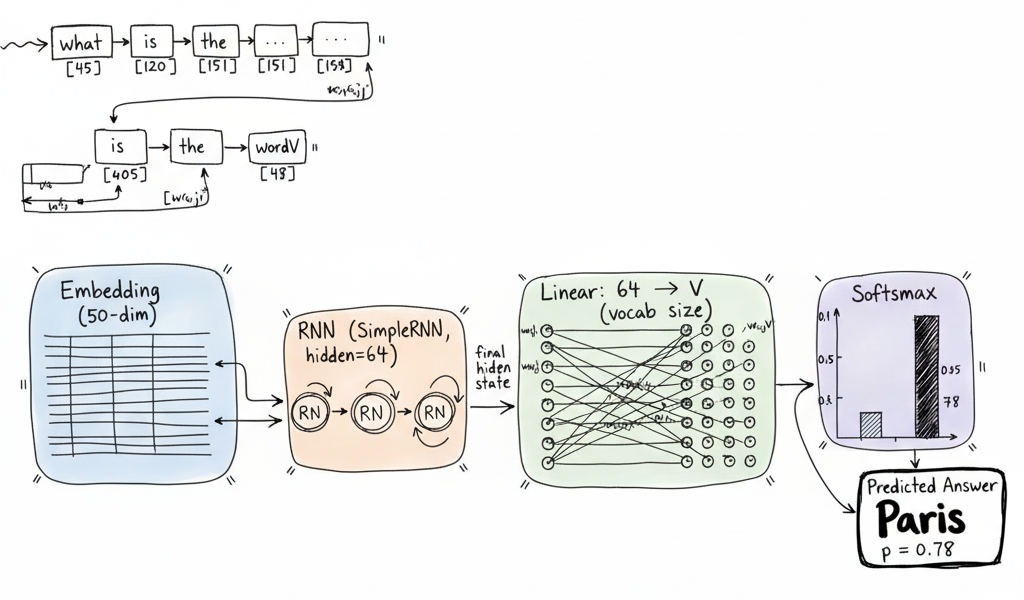
The architecture consists of four main components working in sequence: tokenization converts text into indices, embedding layer maps indices to dense vectors, RNN layer processes the sequence and captures context, and finally a linear layer with softmax produces probability distributions over our vocabulary for answer prediction.

, this tutorial provides a comprehensive overview of RNN fundamentals including architecture details and forward propagation mechanics.

How the Model Actually Works

Let's walk through exactly what happens when someone asks "What is the capital of France?" to understand how each component contributes to getting the answer "Paris".

First, the tokenization process breaks down the question into individual words and converts them into numbers that the computer can understand. The sentence becomes a list of tokens like ["what", "is", "the", "capital", "of", "france"], and each word gets mapped to a specific number from our vocabulary dictionary. Think of this like giving each word in our language a unique ID number.

Next, the embedding layer takes these word IDs and transforms them into rich mathematical representations. Instead of just knowing that "capital" is word number 4, the embedding layer creates a 50-dimensional vector that captures the meaning and relationships of the word "capital" with other words. These embeddings learn that "capital" is related to "city", "country", and "government" through the training process.

The RNN layer is where the magic happens. It processes the question one word at a time, from left to right, building up an understanding of what's being asked. As it reads "what", it starts forming a representation. When it sees "is", it updates its understanding. By the time it processes "capital of France", the RNN has built a comprehensive representation that captures the entire meaning of the question. The final hidden state contains all the context needed to answer the question.

Finally, the linear layer and softmax work together to make the prediction. The linear layer takes the RNN's final understanding and projects it onto our vocabulary size, creating a score for every possible word in our vocabulary. The softmax then converts these scores into probabilities, making the model confident about words like "Paris" while being uncertain about irrelevant words like "elephant". The word with the highest probability becomes our answer.

Why Classification, Not Generation?

This QA system treats answer prediction as a classification problem rather than text generation. Since our dataset contains single-token answers like "Paris" or "Berlin", we can frame this as: "Given a question, which token from our vocabulary is the correct answer?"

This classification approach offers several key advantages that make it perfect for our use case. The training process becomes much simpler because we don't need complex sequence-to-sequence architectures that generate multiple words. Instead, we just need to teach the model to pick the right answer from our vocabulary. The inference is also much faster since a single forward pass through the model produces the answer, rather than generating tokens one by one. We're guaranteed that answers will always come from known tokens in our vocabulary, which prevents the model from making up nonsensical words. Finally, each answer comes with a clear probability score that tells us exactly how confident the model is in its prediction.

Encoder-Only Design Philosophy

Unlike sequence-to-sequence models that need both encoder and decoder, our system uses only an encoder architecture. The question goes through the RNN, and the final hidden state contains all the context needed to predict the answer.

This encoder-only approach works perfectly for our question answering task because we only need single-token outputs rather than generating multi-word responses. The RNN acts as a context compressor, reading through the entire question and squeezing all the important information into its final hidden state. This creates a direct mapping from one compressed representation of the question to one answer token. The computational efficiency is also a major benefit since we need only half the parameters compared to encoder-decoder models, making our system faster to train and run.

Hyperparameter Justification

Embedding Dimension (50): We chose 50 dimensions for our word embeddings because it provides sufficient representation power to capture token relationships without overfitting our relatively small vocabulary of around 100 tokens. This size keeps the model lightweight and memory efficient for our dataset size, while still being large enough to create meaningful representations of word relationships. It's essentially the sweet spot where we get rich enough embeddings without overparameterizing the model.

Hidden State Size (64): The hidden state size of 64 provides enough context capacity to encode patterns from questions of reasonable length. This dimension is intentionally larger than our embedding dimension to allow the RNN to transform and combine the input features effectively. The size also keeps computational costs manageable, ensuring that matrix operations during training and inference remain fast and efficient.

Architecture Comparison

Why Simple RNN over LSTM/GRU? We deliberately chose a simple RNN architecture over more complex LSTM or GRU variants for educational clarity. Understanding the basic RNN mechanics without the complexity of gating mechanisms makes it easier to grasp the core concepts of sequence processing. Our dataset of 100 QA pairs doesn't require the sophisticated memory mechanisms that LSTMs and GRUs provide, and the gradient vanishing problems that these architectures solve are less relevant for the relatively short sequences in our dataset.

Single Layer vs Multi-Layer: A single RNN layer provides sufficient depth to handle the complexity of our question answering task. Adding additional layers would likely cause the model to memorize our small training set rather than learning generalizable patterns, which would hurt performance on new questions. The single-layer approach also makes the model much more interpretable and easier to analyze and debug when things go wrong.

Forward Pass Flow

Let's trace through a concrete example: "What is the capital of France?"

1. Tokenization: ["what", "is", "the", "capital", "of", "france"] → [1, 2, 3, 4, 5, 6]

2. Embedding Lookup: Each index becomes a 50-dimensional vector

   [1] → [0.1, -0.3, 0.8, ...] (50 dims)
   [2] → [0.4, 0.2, -0.1, ...] (50 dims)
   ...
   

3. RNN Processing: Each token vector feeds into the RNN sequentially

   h₀ = [0, 0, ..., 0]           # Initial hidden state (64 dims)
   h₁ = RNN(embed[1], h₀)        # Process "what"
   h₂ = RNN(embed[2], h₁)        # Process "is"
   h₃ = RNN(embed[3], h₂)        # Process "the"
   ...
   h₆ = RNN(embed[6], h₅)        # Process "france" → final state
   

4. Linear Projection: Final hidden state h₆ projects to vocabulary size

   logits = Linear(h₆)           # [64] → [vocab_size]
   

5. Softmax & Prediction: Convert logits logits to probabilities

   probabilities = softmax(logits)
   predicted_token = argmax(probabilities)  # Index 7 → "paris"
   

The beauty of this architecture lies in its simplicity: the RNN accumulates context as it processes each word, and by the final token, it has built a representation that encodes the entire question's meaning, ready for classification.

Model Instantiation and Setup

With our architecture defined, creating the model is straightforward. The key parameter is the vocabulary size, which determines our output dimensions:

import torch
import torch.nn as nn

class SimpleRNN(nn.Module):
    def __init__(self, vocab_size, embedding_dim=50, hidden_size=64):
        super(SimpleRNN, self).__init__()
        self.embedding = nn.Embedding(vocab_size, embedding_dim)    # Token → dense vectors
        self.rnn = nn.RNN(embedding_dim, hidden_size, batch_first=True)  # Sequential processing
        self.fc = nn.Linear(hidden_size, vocab_size)                # Final classification layer

    def forward(self, x):
        embedded = self.embedding(x)                    # [batch, seq_len] → [batch, seq_len, embed_dim]
        rnn_out, hidden = self.rnn(embedded)           # Process sequence
        final_output = rnn_out[:, -1, :]               # Take last timestep [batch, hidden_size]
        logits = self.fc(final_output)                 # Project to vocab size [batch, vocab_size]
        return logits

# Initialize the model
vocab_size = len(vocab)  # Total unique tokens in our vocabulary
model = SimpleRNN(vocab_size=vocab_size)
print(f"Model created with vocabulary size: {vocab_size}")

Memory and scalability considerations:

• Parameter count: ~(vocab_size × 50) + (50 × 64) + (64 × 64) + (64 × vocab_size) ≈ 2 × vocab_size × 114 parameters
• Memory footprint: For our ~100 token vocabulary, this results in roughly 23K parameters - lightweight and manageable
• Scalability: Linear growth with vocabulary size makes this approach suitable for controlled domains but challenging for large, open vocabularies

Training Process and Optimization

Dataset Preparation

PyTorch's Dataset and DataLoader classes provide a clean abstraction for feeding data to our model. Here's our custom dataset implementation:

from torch.utils.data import Dataset, DataLoader
import torch

class QADataset(Dataset):
    def __init__(self, dataframe, vocab, tokenize_fn):
        self.data = dataframe                          # Store the Q&A pairs
        self.vocab = vocab                             # Token → index mapping
        self.tokenize = tokenize_fn                    # Text preprocessing function

    def __len__(self):
        return len(self.data)                          # Required by PyTorch Dataset

    def __getitem__(self, idx):
        row = self.data.iloc[idx]                      # Get specific Q&A pair
        question = row['question']                     # Extract question text
        answer = row['answer']                         # Extract answer text

        # Convert text to indices
        question_indices = self.text_to_indices(question)
        answer_index = self.vocab.get(answer.lower(), self.vocab['<UNK>'])  # Single token answer

        return torch.tensor(question_indices), torch.tensor(answer_index)

    def text_to_indices(self, text):
        tokens = self.tokenize(text)                   # Tokenize the input text
        indices = [self.vocab.get(token, self.vocab['<UNK>']) for token in tokens]  # Map to indices
        return indices

# Create dataset and dataloader
dataset = QADataset(df, vocab, tokenize)
dataloader = DataLoader(dataset, batch_size=1, shuffle=True)  # batch_size=1 for simplicity

Why batch_size=1?

• Variable sequence lengths: Questions have different lengths, and batch_size=1 avoids padding complexity
• Educational clarity: Easier to understand the training process without batching overhead
• Small dataset: With only 100 examples, larger batches don't provide significant computational benefits
• Memory efficiency: Minimal memory requirements for our lightweight model

Data shuffling importance:

• Prevents overfitting: Randomizes the order each epoch, reducing memorization of training sequence
• Better convergence: Helps the optimizer explore different gradient directions
• Robust learning: Model learns patterns rather than data ordering artifacts

Loss Function and Optimizer Selection

The choice of loss function and optimizer directly impacts training effectiveness. Here's our setup and reasoning:

import torch.optim as optim
import torch.nn.functional as F

# Loss function: CrossEntropyLoss for multi-class classification
criterion = nn.CrossEntropyLoss()

# Optimizer: Adam with learning rate 0.001
optimizer = optim.Adam(model.parameters(), lr=0.001)

Why CrossEntropyLoss? CrossEntropyLoss is perfect for our classification task because:

• Multi-class classification: Each answer is one token from our vocabulary (mutually exclusive classes)
• Probability interpretation: Softmax + negative log-likelihood provides clear confidence scores
• Gradient flow: Well-behaved gradients help with training stability
• Built-in efficiency: PyTorch optimizes this combination computationally

Classification vs Language Modeling Connection: While traditional language models predict the next token in a sequence, our system predicts the answer token given a complete question. This is essentially a conditional classification problem where:

• Input: Complete question sequence
• Output: Single answer token (class)
• Objective: Maximize probability of correct answer token

Adam vs SGD Choice: Adam optimizer offers several advantages for our use case:

• Adaptive learning rates: Different parameters get different learning rates based on gradient history
• Momentum-like behavior: Helps escape local minima with exponential moving averages
• Less hyperparameter tuning: Works well with default parameters (β₁=0.9, β₂=0.999)
• Fast convergence: Particularly effective for small datasets like ours

Learning Rate Selection (0.001):

• Conservative starting point: 0.001 is a safe default that rarely causes training instability
• Small dataset consideration: Lower learning rates prevent rapid overfitting to our 100 examples
• Fine-tuning strategy: Can be reduced by factor of 10 if loss plateaus (0.0001) or increased if training is too slow (0.01)

Training Loop Implementation

Now comes the core training process. Here's the complete training loop with detailed explanations:

learning_rate = 0.001
epochs = 20

model = SimpleRNN(len(vocab))
criterion = nn.CrossEntropyLoss()
optimizer = torch.optim.Adam(model.parameters(), lr=learning_rate)

# Training loop
for epoch in range(epochs):
    total_loss = 0                                     # Track cumulative loss per epoch

    for question, answer in dataloader:               # Iterate through Q&A pairs
        optimizer.zero_grad()                         # Clear gradients from previous step

        # Forward pass
        output = model(question)                      # Get model predictions [1, vocab_size]

        # Loss calculation -> output shape (1,324) vs answer shape (1)
        loss = criterion(output, answer[0])           # Compare prediction with true answer

        # Backpropagation
        loss.backward()                               # Compute gradients via chain rule

        # Parameter update
        optimizer.step()                              # Apply gradients to update weights

        total_loss = total_loss + loss.item()         # Accumulate loss for monitoring

    print(f"Epoch: {epoch+1}, Loss: {total_loss:.4f}")

Training Process Breakdown: The training process follows a systematic cycle that repeats for each question-answer pair. We start with a gradient reset using zero_grad() because PyTorch accumulates gradients by default, so we need to clear them from the previous iteration. Then comes the forward pass where the question flows through the embedding layer, then the RNN, and finally the linear layers to produce predictions. The loss calculation uses CrossEntropyLoss to compare the model's output probabilities with the true answer index, measuring how far off our prediction was. The backward pass uses automatic differentiation to compute gradients for all parameters throughout the network, calculating exactly how much each weight contributed to the error. Finally, the Adam optimizer adjusts all the weights based on these computed gradients, moving the model closer to the correct answer.

Training Expectations: During the initial epochs, you should see the loss decrease rapidly from around 5.8, which represents random chance performance with our vocabulary size of about 324 tokens. The model typically converges with the loss stabilizing around 0.1 to 1.0 after 10-15 epochs, indicating that it has learned the patterns in our training data. Watch out for overfitting signs where the loss approaches 0, as this usually indicates the model is memorizing the training examples rather than learning generalizable patterns. The entire training process should take only 1-2 minutes on a CPU for 20 epochs given our small dataset size.

Inference and Prediction

With training complete, we can now use our model to answer questions. The prediction pipeline transforms raw text questions into confidence-scored answers.

Prediction Pipeline Implementation

Here's our complete prediction function that handles the full inference pipeline:

def predict(model, question, threshold=0.5):
    # Step 1: Convert question to numerical indices
    numerical_question = text_to_indices(question, vocab)

    # Step 2: Create tensor with batch dimension
    question_tensor = torch.tensor(numerical_question).unsqueeze(0)  # [1, seq_len]

    # Step 3: Get model output (logits)
    output = model(question_tensor)                                  # [1, vocab_size]

    # Step 4: Convert logits to probabilities
    probs = torch.nn.functional.softmax(output, dim=1)               # Normalize to [0,1]

    # Step 5: Find highest confidence prediction
    value, index = torch.max(probs, dim=1)                          # Get max prob & index

    # Step 6: Apply confidence threshold
    if value < threshold:
        return "I don't know"                                        # Low confidence

    # Step 7: Convert index back to token
    predicted_token = list(vocab.keys())[index]
    return predicted_token

# Test the model
result = predict(model, "What is the largest planet in our solar system?")
print(result)  # Expected: "jupiter"

Pipeline Step Analysis:

1. Text Preprocessing: Uses same tokenization as training for consistency
2. Tensor Conversion: Adds batch dimension for model compatibility
3. Model Inference: Single forward pass produces raw scores
4. Probability Conversion: Softmax ensures interpretable confidence scores
5. Confidence Checking: Threshold guards against uncertain predictions
6. Answer Decoding: Maps numerical prediction back to human-readable text

Confidence Thresholding Strategy

The confidence threshold (default 0.5) acts as a quality gate for predictions:

Why Thresholding Matters: Confidence thresholding is crucial for building reliable AI systems because it prevents the model from giving confident-sounding wrong answers, which can be more dangerous than admitting uncertainty. Users develop much more trust in systems that say "I don't know" rather than providing incorrect information with false confidence. The threshold also helps the model understand its own training boundaries and stay within its area of expertise.

Threshold Tuning Considerations: Different threshold values create different behavior patterns that suit various applications. A high threshold of 0.8 or above creates very conservative behavior with fewer but more accurate answers, perfect for critical applications where wrong information could be harmful. A medium threshold between 0.5 and 0.7 provides a balanced approach with reasonable coverage and good accuracy, suitable for most general-purpose applications. A low threshold of 0.3 or below enables liberal answering with higher coverage but more errors, which might work for exploratory or educational contexts where engagement matters more than perfect accuracy.

Real-world Applications: Different use cases require different threshold strategies. Customer service chatbots might use high thresholds to avoid misinformation, while educational tools might use lower thresholds to encourage exploration.

Practical Usage Examples

Let's test our model with various questions to understand its behavior:

# Test cases demonstrating model capabilities and limitations
test_questions = [
    "What is the capital of France?",           # Training data - should work
    "What is the capital of Germany?",          # Training data - should work
    "What is the largest planet?",              # Slight variation - might work
    "Who is the president of USA?",             # Outside training - should say "I don't know"
]

for question in test_questions:
    answer = predict(model, question, threshold=0.5)
    print(f"Q: {question}")
    print(f"A: {answer}\n")

Expected Behavior Patterns: The model exhibits predictable behavior patterns based on how closely questions match its training data. Questions that are similar to training examples get confident and correct answers because the model recognizes familiar patterns. Slight phrase variations may still work if the key tokens are preserved, as the model can often generalize to different phrasings of the same question. Completely different topics that are outside the training domain typically trigger "I don't know" responses, which is exactly what we want for reliability. In-domain questions usually score confidence levels of 0.7 to 0.9 or higher, while out-of-domain questions score much lower.

Performance Evaluation and Analysis

Model Performance Analysis

Our RNN QA system demonstrates solid performance on the training dataset while revealing important limitations that inform future improvements.

Training Set Accuracy:

# Simple accuracy evaluation on training data
def evaluate_model(model, dataloader, vocab):
    correct_predictions = 0
    total_questions = 0

    with torch.no_grad():  # Disable gradient computation for evaluation
        for question, answer in dataloader:
            output = model(question)
            predicted_index = torch.argmax(output, dim=1)

            if predicted_index.item() == answer[0].item():
                correct_predictions += 1
            total_questions += 1

    accuracy = correct_predictions / total_questions
    return accuracy

training_accuracy = evaluate_model(model, dataloader, vocab)
print(f"Training Accuracy: {training_accuracy:.2%}")

Expected Performance:

• Training accuracy: 85-95% after 20 epochs
• High confidence predictions: ~90% accuracy
• Low confidence cases: Model appropriately says "I don't know"

Error Pattern Analysis:

1. Token Mismatch Errors: Questions with slight word variations ("What's" vs "What is") may fail
2. Context Confusion: Complex questions with multiple entities can confuse the single-output constraint
3. Vocabulary Gaps: Any word not in training vocabulary defaults to <UNK>, potentially breaking understanding
4. Sequence Length Sensitivity: Very short or very long questions may challenge the RNN's context encoding

Model Behavior Insights:

• Question Types: "What is the..." patterns work best due to training data structure
• Confidence Correlation: Shorter, direct questions typically yield higher confidence scores
• Robustness: Model handles minor punctuation and case variations well due to preprocessing

Limitations and Modern Alternatives

Architectural Limitations

Single-Token Output Constraint: Our model can only predict one answer token, severely limiting response complexity. Real-world questions often require multi-word answers, explanations, or contextual responses.

Sequential Processing Inefficiency: RNNs process tokens one-by-one, making them slower than transformer architectures that can parallelize attention across the entire sequence. This becomes problematic for longer questions.

Context Window Limitations: Simple RNNs struggle with long-range dependencies. Important context from early in a question may be "forgotten" by the time the model reaches the end, especially without gating mechanisms like LSTM/GRU.

Vocabulary Scalability: Our approach scales linearly with vocabulary size in both memory (embeddings) and computation (final linear layer). Real-world applications with 50K+ vocabularies become computationally expensive.

Dataset and Scope Constraints

Limited Generalization: With only 100 training examples, our model essentially memorizes question-answer patterns rather than learning genuine language understanding. This prevents generalization to novel questions.

Domain Specificity: Our model knows only what's in the training data. It has no world knowledge, common sense reasoning, or ability to handle questions outside its narrow scope.

No Multi-Step Reasoning: Complex questions requiring inference, calculation, or logical reasoning are beyond this architecture's capabilities. The model can only perform direct pattern matching.

Modern Alternatives and Evolution

Transformer Advantages:

• Parallel Processing: All tokens processed simultaneously via self-attention
• Long-Range Dependencies: Attention mechanism directly connects distant tokens
• Scalability: Better performance scaling with model size and data

Pre-trained Model Benefits:

• Transfer Learning: Models like BERT/GPT leverage massive pre-training
• World Knowledge: Broad understanding from internet-scale training
• Few-Shot Learning: Can adapt to new tasks with minimal examples

Advanced Approaches:

• Sequence-to-Sequence: Generate multi-token responses
• Retrieval-Augmented Generation (RAG): Combine parametric knowledge with external retrieval
• Large Language Models: GPT-3/4 class models handle complex reasoning and generation

Conclusion

We've built a complete RNN-based question answering system from scratch, covering every step from data preprocessing to model deployment considerations. While our simple architecture has clear limitations compared to modern transformer-based systems, it provides invaluable insights into the foundational concepts that power today's AI.

Key Technical Achievements: We've accomplished several important technical milestones in building this system. We created a complete end-to-end pipeline that takes raw text and transforms it into a working QA system that can answer questions and provide confidence scores. Our vocabulary management system dynamically maps tokens with proper unknown word handling, creating a robust foundation for text processing. The neural architecture follows a clean embedding to RNN to classification pipeline that's both understandable and effective. We implemented a complete training process with optimization loops and loss monitoring that demonstrates proper machine learning practices. Finally, we built an inference system with confidence-based prediction and intelligent fallback handling that makes the system practical for real-world use.

Educational Value: This project demonstrates core NLP concepts that remain relevant across all modern architectures. Understanding how RNNs process sequences, how embeddings represent meaning, and how classification works at the token level provides the foundation for grasping more complex systems like GPT and BERT.

Connection to Modern NLP: The concepts we've learned here connect directly to cutting-edge NLP technologies. Transformers build on these same sequence modeling concepts but replace recurrence with attention mechanisms for better parallelization and long-range dependencies. Large Language Models like GPT use similar token prediction approaches but operate at massive scale with sophisticated training techniques and billions of parameters. RAG Systems combine our retrieval concepts with generation capabilities, allowing models to access external knowledge while generating responses. Fine-tuning approaches extend our domain adaptation ideas to pre-trained models, allowing massive models to specialize for specific tasks with relatively little additional training data.

Next Steps for Exploration: There are many exciting directions to take this project further. Start by experimenting with LSTM/GRU variants and comparing their performance to understand how gating mechanisms improve sequence modeling. Expand the dataset to 1000+ Q&A pairs and observe how generalization improves with more training data. Implement attention mechanisms to understand the foundations of transformer architectures and see how focusing on relevant parts of questions improves answers. Try multi-token generation for more complex answers that go beyond single-word responses. Finally, explore modern frameworks like Hugging Face Transformers to see how the concepts you've learned here apply to state-of-the-art models.

The beauty of starting with simple architectures is that every concept scales up. The vocabulary building, training loops, and inference patterns you've learned here apply directly to state-of-the-art models – they just operate at larger scales with more sophisticated architectures.

Building this RNN QA system gives you the conceptual foundation to understand, modify, and create the next generation of AI systems. Start simple, understand deeply, then scale up.

Available for hire - If you're looking for a skilled full-stack engineer with expertise in AI integration, feel free to reach out at hire@codewarnab.in